---
title: "Introduction to Statistical Methods"
subtitle: "Week 1"
date: 2025-04-03
format:
html:
embed-resources: true
toc: true
---
# Before we start
artur-baranov.github.io/nu-ps312-ds
```{r}
#| warning: false
library(qrcode)
qr_code('https://artur-baranov.github.io/nu-ps312-ds') |>
plot()
```
## Getting to know each other
First of all, introduction time!
- Your name
- Your interest in the political science
- Your previous experience with R
## Agenda
- Getting used to work in RStudio
- Loading data into R
- Practicing asking statistical questions
# Introduction to the DS & Software
## How we work
- Create a folder for the PS312 discussion section.
- Download the script and the data, and put them into the created folder.
- Follow the script throughout the discussion section, run the code.
- Explore the syntax. Amend the code after the class, play with graphs and functions. Experiment!
You can install R and RStudio, instructions are available [here](https://artur-baranov.github.io/nu-ps312-ds/ps312-d_00.html). Alternatively, feel free to use [Posit.Cloud](https://posit.cloud/)
## Navigating RStudio
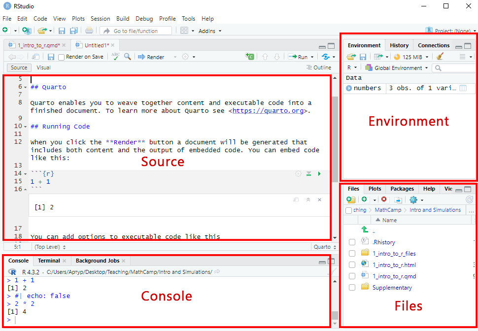
It will take some time to understand how everything works in RStudio, but once you understand it, it’s quite straightforward. The most classic UI consists of four panes.
- **Source**. Here we write code to run and text.
- **Environment**. This pane allows you to interact with the data loaded into RStudio.
- **Console**. This pane provides an area to interactively execute code.
- **Files**. By default, this pane has your working directory. From here you can access files associated with the project.
# Programming
## Code Chunk
To insert a **Code Chunk**, you can use `Ctrl+Alt+I` on Windows and `Cmd+Option+I` on Mac. Run the whole chunk by clicking the green triangle, or one/multiple lines by using `Ctrl + Enter` or `Command + Return` on Mac.
```{r}
print("Code Chunk")
```
::: {.callout-tip icon="false"}
## Coding Task
Insert a chunk. Print "Northwestern".
:::
## Function and Arguments
Most of the **functions** we want to run require an **argument**. For example, the function `print()` above takes the argument "Code Chunk".
```{r}
#| eval: false
function(argument)
```
## Pipes
**Pipes** (`%>%` or `|>`) are helpful for streamlining the coding. They introduce linearity to the process of writing the code. In plain English, a pipe translates to "take an object, and then".
```{r}
numbers = c(1, 2, 3) # a vector object
numbers |>
print()
```
## Libraries
Quite often we rely on non-native functions. To use them, we need to first install and then load libraries. Let's do it step-by-step,
Firstly, let's install a package `tidyverse`. Run the chunk below only once! Generally, it's considered to be a good manner to remove `install.packages()` command from scripts.
```{r}
#| eval: false
install.packages("tidyverse")
```
Make sure you removed the chunk with `install.packages()` function. Now, load the library to the current R session. We'll be working with this library extensively throughout the quarter.
```{r}
#| message: false
library(tidyverse)
```
# Asking Questions
Today we are working with the World Happiness Report. The [codebook](https://happiness-report.s3.amazonaws.com/2024/Ch2+Appendix.pdf) is here to help us - it's quite useful to search for one when dealing with third party data. Here are some variables listed in the codebook:
- `Country_name` is the name of the country
- `Ladder_score` is the happiness score
- `Logged_GDP_per_capita` is the log of GDP per capita
And many others.
Let's load the data.
```{r}
#| message: false
whr = read_csv("data/WHR.csv")
```
To print first 6 rows in the dataset you can use `head()` function.
```{r}
head(whr)
```
## Exctracting Facts from the Data
Often we start with descriptive questions.
What is the happiest country?
```{r}
whr %>%
select(Country_name, Ladder_score) %>% # choosing the variables
arrange(-Ladder_score) %>% # arranging data in descending order
head(1) # leaving the first observation
```
What is the least happy country?
```{r}
whr %>%
select(Country_name, Ladder_score) %>% # choosing the variables
arrange(Ladder_score) %>% # arranging data in ascending order
head(1) # leaving the first observation
```
How happy are the countries?
```{r}
ggplot(data = whr) +
geom_histogram(aes(x = Ladder_score))
```
These questions allow us to be informed only about the 'facts' or the data we are working with. Though quite descriptive, they provide some intuition about what's happening. What are some potentially intriguing patterns you observe in the graph above?
## Relationships between the variables
Let's start to explore more interesting patterns. Regularly, the starting point is a normative question. For example, **how to make our country happier?**.
::: {.callout-note icon="false"}
## Qustion
1. How would you answer this question and what would you need to answer this question?
2. Think through the question, how can you make it a statistical research question?
:::
We are researching causal relations. But on initial steps, we quite often start with correlations. Let's focus on the relationship between happinness and wealth measured as GDP.
::: {.callout-note icon="false"}
## Qustion
What type of the relationship is between Happiness and Wealth? Is it strong? What is the direction?
```{r}
cor(whr$Ladder_score, whr$Logged_GDP_per_capita)
```
:::
Let's visualize this relationship.As a rule of thumb, when speaking about a relationship whose causal nature we have not definitively determined, we say there is an association between X and Y. Is there one?
```{r}
#| message: false
ggplot(data = whr, aes(x = Logged_GDP_per_capita, y = Ladder_score)) +
geom_point() +
geom_smooth(method = "lm") +
labs(x = "Wealth",
y = "Happiness")
```
## Tips for Thinking About Statistical Relationships
- Ask yourself: what are you interested in? Then, identify what is your dependent (i.e., what are you explaining) and independent variables (i.e., what is the explanatory factor).
- Do not underestimate the exploratory analysis. Explore your data! Get as much information as possible, find patterns and explore the relations between various variables of your interest
- Think about causality. Are you sure that your independent variable causes change in dependent variable?
# Check List
I know how to insert a chunk of code and run it
I know how directories work and how to load data in R
I am familiar with concept of independent and dependent variables
I am starting to understand how to ask statistical research questions, and the word causality does not scare me