library(tidyverse)
library(readxl)
cpds = read_excel("data/cpds.xlsx")Data Wrangling and Classes
Week 2
Before we start
- Any questions?
Review of the Previous Session
Let’s refresh what we did last week.
Review
First of all, let’s load the tidyverse and readxl libraries. Then, load the Comparative Political Dataset from the last class.
Imagine you are interested in fractionalizon of electoral systems (you can read more about fractionalization after class here). Subset the following variables from the dataset: year, country, rae_ele and fed.
cpds_subset = cpds ...
...(year, ...)Rename the rae_ele to fractionalization in the cpds_subset dataframe.
... = cpds_subset %>%
...(fractionalization = ...)Draw a histogram to show the distribution of Douglas Rae’s index of electoral fractionalization.
... +
geom_histogram(...)What is the minimum value? What is the maximum value?
...The index indicates that 1 corresponds to a fragmented system (votes are widely dispersed across parties), while 0 means that everyone voted for the same party. What is the average?
Draw a geom_boxplot() to see the relationship between the federalism (fed) on the x axis and fractionalization on the y axis. The federalism is coded as: 0 = no; 1 = weak; 2 = strong. Is something wrong?
...
...(aes(...))Don’t forget to remove the cpds and cpds_subset dataframes.
rm(cpds, cpds_subset)Agenda for Today
Data Classes
Data Wrangling
Presenting data with
tinytable
Exploring and Wrangling Data
Let’s load the data
load(url("https://github.com/vdeminstitute/vdemdata/raw/6bee8e170578fe8ccdc1414ae239c5e870996bc0/data/vdem.RData"))This is the V-Dem dataset. For your reference, their codebook is available here.
The dataset is huge! Be careful
nrow(vdem)
ncol(vdem)[1] 27734
[1] 4607Imagine you are interested in the relationship between regime type and physical violence. Let’s select() and rename the variables we will work with. Quite unfortunately, the names of the variables are not as straightforward. The regime index is e_v2x_polyarchy_5C and Physical violence index is v2x_clphy. And you can combine both actions in the same function!
violence_data = vdem %>%
select(country_name,
year,
regime = e_v2x_polyarchy_5C,
violence = v2x_clphy) Let’s see the result
head(violence_data) country_name year regime violence
1 Mexico 1789 0 0.322
2 Mexico 1790 0 0.322
3 Mexico 1791 0 0.322
4 Mexico 1792 0 0.322
5 Mexico 1793 0 0.322
6 Mexico 1794 0 0.322That was the first step. Let’s subset even more data. Let’s analyze the distribution of the Violence Index in the year 2000. We need to filter the data for this task.
violence_2000 = violence_data %>%
filter(year == 2000)The higher the number, the better the physical integrity in a given country.
ggplot(data = violence_2000) +
geom_histogram(aes(x = violence))
Let’s customize the plot a bit.
ggplot(data = violence_2000) +
geom_histogram(aes(x = violence)) +
labs(title = "Physical Integrity Rights Index",
subtitle = "In 2000",
x = "Violence Integrity Index",
y = "") +
theme_bw()`stat_bin()` using `bins = 30`. Pick better value `binwidth`.
Imagine, you asked the following question. Is it true that in the year 2000 democracies had better violence integrity rights index?
Firstly, you we need to differentiate between the regimes. Using mutate() function we can create and modify existing variables. Let’s do that!
violence_2000 = violence_2000 %>%
mutate(democracy = case_when(regime >= 0.5 ~ "Democracy",
regime < 0.5 ~ "Autocracy"))
head(violence_2000) country_name year regime violence democracy
1 Mexico 2000 0.75 0.573 Democracy
2 Suriname 2000 0.75 0.871 Democracy
3 Sweden 2000 1.00 0.990 Democracy
4 Switzerland 2000 1.00 0.974 Democracy
5 Ghana 2000 0.75 0.946 Democracy
6 South Africa 2000 0.75 0.834 DemocracyThere are multiple ways to visually compare between two groups.
Let’s draw histograms first.
ggplot(violence_2000) +
geom_histogram(aes(x = violence, fill = democracy))
But comparing distributions between groups is easier with the boxplot. Are they different?
ggplot(violence_2000) +
geom_boxplot(aes(x = democracy, y = violence))
Data Classes
You can represent the same concepts with numbers or characters. For example, we have two variables indicating the regime type. One of which is more granular, regime. Another is binary, which is democracy. Explore the latter first.
with(violence_2000,
table(regime))regime
0 0.25 0.5 0.75 1
32 45 33 30 37 Now, explore the former. Side note, pay attention to syntax, the functions are almost equivalent.
table(violence_2000$democracy)
Autocracy Democracy
77 100 Theoretically, we can plot even more detailed graph using geom_boxplot() if we use regime data. Let’s see. Something fails!
ggplot(violence_2000) +
geom_boxplot(aes(x = regime, y = violence))Warning: Continuous x aesthetic
ℹ did you forget `aes(group = ...)`?
Let’s correct. Now it’s better!
ggplot(violence_2000) +
geom_boxplot(aes(x = as.factor(regime), y = violence))
The problem is, by default R treats regime variable as continuous, but it’s categorical! Explore the graph below.
library(DiagrammeR)
mermaid("
graph LR
D[Data] --> C[Categorical]
D --> N[Numerical]
C --> no[Nominal]
C --> Or[Ordinal]
N --> di[Discrete]
N --> co[Continuous]
no --> c[Character]
Or --> f[Factor]
di --> i[Integer]
co --> n[Numeric]
")These are the basic classes of data in R. Some examples might include:
Nominal: Names, Labels, Brands, Country names, etc.
Ordinal: Educational Levels (High School-BA-MA-PhD), Customer Rating (Unsatisfied-Neutral-Satisfied), etc.
Discrete: Number of customers per day, number of seats won by political parties, etc.
Continuous: Height of people, voter turnout, etc.
You can check the class using class() function.
class(violence_2000$regime)[1] "numeric"And you can make it categorical by transforming it to factor using as.factor(). Other functions are as.numeric()and as.character().
violence_2000$regime = as.factor(violence_2000$regime)Summarizing and Presenting data
Treating a variable as categorcal would help us to summarize data per category. For example, you want to present information of average level of violence in different regimes.
Let’s switch to the main dataset. Quickly prepare the data using case_when() function – a better version of ifelse(). Here we are using the codebook’s guidence to rename the categories.
violence_data = violence_data %>%
mutate(regime = case_when(regime > 0.75 ~ "Democratic",
regime == 0.75 ~ "Minimally Democratic",
regime == 0.5 ~ "Ambivalent",
regime == 0.25 ~ "Autocratic",
regime < 0.25 ~ "Closed Autocratic"))
head(violence_data) country_name year regime violence
1 Mexico 1789 Closed Autocratic 0.322
2 Mexico 1790 Closed Autocratic 0.322
3 Mexico 1791 Closed Autocratic 0.322
4 Mexico 1792 Closed Autocratic 0.322
5 Mexico 1793 Closed Autocratic 0.322
6 Mexico 1794 Closed Autocratic 0.322A tricky but helpful operation is groupping a variable, and then calculating statistics. This picture really helps me wrap my head around it.
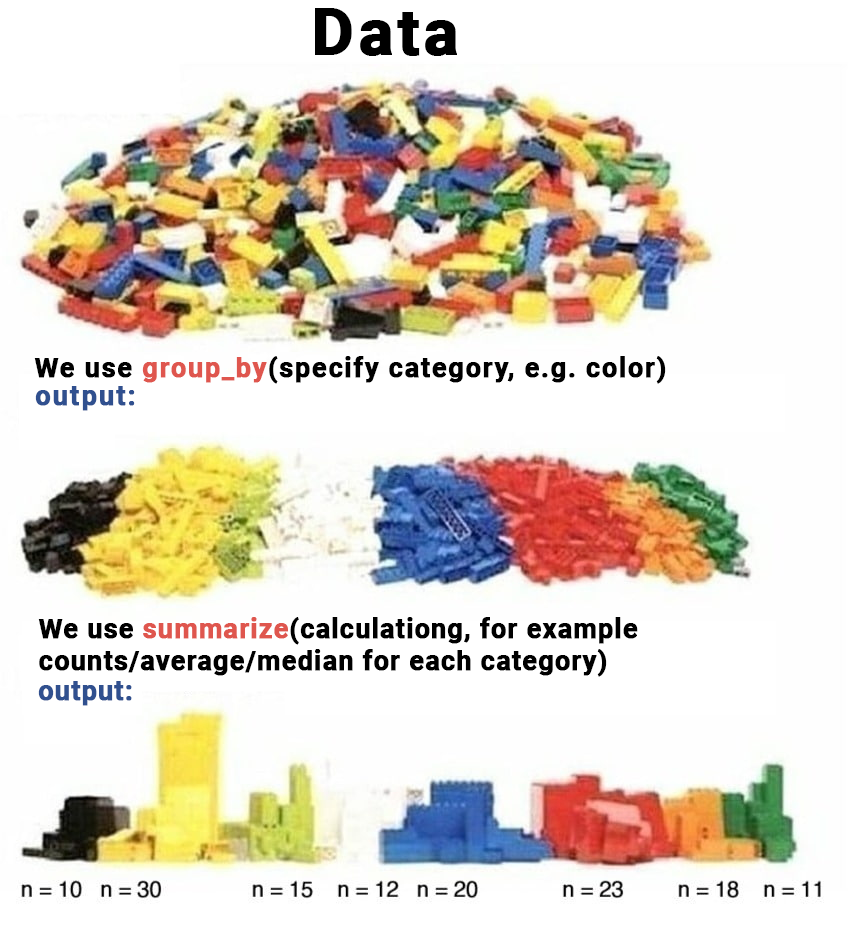
regime_violence = violence_data %>%
group_by(regime) %>%
summarize(average = mean(violence, na.rm = TRUE))
regime_violence# A tibble: 6 × 2
regime average
<chr> <dbl>
1 Ambivalent 0.733
2 Autocratic 0.584
3 Closed Autocratic 0.361
4 Democratic 0.955
5 Minimally Democratic 0.874
6 <NA> 0.466Finally, let’s present that in a nice way using tinytable library.
library(tinytable)
regime_violence %>%
tt(title = "Average level of violence in different regimes")| regime | average |
|---|---|
| Ambivalent | 0.7333526 |
| Autocratic | 0.5838729 |
| Closed Autocratic | 0.3613431 |
| Democratic | 0.9548574 |
| Minimally Democratic | 0.8740276 |
| NA | 0.4657441 |
Check list
Optional Exercises
Create a new violence_2010 dataset, by subsetting violence_data for year 2010.
Using mutate() and case_when(), create a new variable violence_binary that is “High integrity” if the violence variable is greater or equal to 0.5, and “Low integrity” if it is less than 0.5.
Compare the two variables coding: violence and violence_binary. Check there classes. What is the difference? Briefly describe the type of each variable. Imagine you were to draw a boxplot, how would class differences in the variables define their use case on the graph?
Let’s calculate the average regime type per violence_binary. Use group_by() and summarize(). Save it to output object.
Using tt() present the output.