---
title: "Last Quarter's Review"
subtitle: "Week 1"
date: 2025-01-09
format:
html:
embed-resources: true
toc: true
---
# Before we start
- We are expected to have installed R and RStudio, if not see the [installing R section](#installingr).
- In the discussion section, we will focus on coding and practicing what we have learned in the lectures.
- Office hours are on Tuesday, 11-12:30 Scott 110.
- Questions?
Download script
# Brief recap of the last quarter
## Coding Terminology
### Code Chunk
To insert a **Code Chunk**, you can use `Ctrl+Alt+I` on Windows and `Cmd+Option+I` on Mac. Run the whole chunk by clicking the green triangle, or one/multiple lines by using `Ctrl + Enter` or `Command + Return` on Mac.
```{r}
print("Code Chunk")
```
### Function and Arguments
Most of the **functions** we want to run require an **argument** For example, the function `print()` above takes the argument "Code Chunk".
```{r}
#| eval: false
function(argument)
```
### Data structures
There are many **data structures**, but the most important to know the following.
- **Objects.** Those are individual units, e.g. a number or a word.
```{r}
#| results: hold
number = 1
number
word = "Northwestern"
word
```
- **Vectors**. Vectors are collections of objects. To create one, you will need to use function `c()`.
```{r}
numbers = c(1, 2, 3)
numbers
```
- **Dataframes**. Dataframes are the most used data structure. Last quarter you spend a lot of time working with it. It is a table with data. Columns are called variables, and those are vectors. You can access a column using `$` operator.
```{r}
#| results: hold
df = data.frame(numbers,
numbers_multiplied = numbers * 2)
df
df$numbers_multiplied
```
### Data classes
We work with various **classes of data**, and the analysis we perform depends heavily on these classes.
- **Numeric**. Continuous data.
```{r}
#| results: hold
numeric_class = c(1.2, 2.5, 7.3)
numeric_class
class(numeric_class)
```
- **Integer**. Whole numbers (e.g., count data).
```{r}
#| results: hold
integer_class = c(1:3)
class(integer_class)
```
- **Character**. Usually, represent textual data.
```{r}
word
class(word)
```
- **Factor**. Categorical variables, where each value is treated as an identifier for a category.
```{r}
#| results: hold
colors = c("blue", "green")
class(colors)
```
As you noticed, R did not identify the class of data correctly. We can change it using `as.factor()` function. You can easily change the class of your variable (`as.numeric()`, `as.integer()`, `as.character()`)
```{r}
colors = as.factor(colors)
class(colors)
```
### Libraries
Quite frequently, we use additional **libraries** to extend the capabilities of R. I'm sure you remember `tidyverse`. Let's load it.
```{r}
#| message: false
library(tidyverse)
```
If you updated your R or recently downloaded it, you can easily install libraries using the function `install.packages()`.
### Pipes
**Pipes** (`%>%` or `|>`) are helpful for streamlining the coding. They introduce linearity to the process of writing the code. In plain English, a pipe translates to "take an object, and then".
```{r}
numbers %>%
print()
```
# Describing Data
First task, let's load the data
```{r}
load(url("https://github.com/vdeminstitute/vdemdata/raw/6bee8e170578fe8ccdc1414ae239c5e870996bc0/data/vdem.RData"))
```
This is the V-Dem dataset. For your reference, their codebook is available [here](https://v-dem.net/documents/38/V-Dem_Codebook_v14.pdf).
The dataset is huge! Be careful
```{r}
#| results: hold
nrow(vdem)
ncol(vdem)
```
Imagine you are interested in the relationship between regime type and physical violence. Let’s **select** the variables we will work with. Quite unfortunately, the names of the variables are not as straightforward. The regime index is `e_v2x_polyarchy_5C` and Physical violence index is `v2x_clphy`.
```{r}
violence_data = vdem %>%
select(country_name, year, e_v2x_polyarchy_5C, v2x_clphy)
```
Let's **rename** the variables so it's easier to work with them.
```{r}
violence_data = violence_data %>%
rename(regime = e_v2x_polyarchy_5C,
violence = v2x_clphy)
head(violence_data)
```
Now, analyze the regime data. We can describe regime data using various statistics. Let's check the min score for the regime.
```{r}
min(violence_data$regime, na.rm = T)
```
Check the max score for the regime variable below.
```{r}
#| eval: false
...(violence_data$regime, na.rm = T)
```
Check the average score for the regime variable below.
```{r}
#| eval: false
mean(..., na.rm = T)
```
Finally, use the `summary()` function to get the descriptive statistics.
```{r}
summary(violence_data$regime)
```
::: callout-note
## Exercise
Select country name (`contry_name`), year (`year`) and Political corruption index (`v2x_corr`) from the `vdem` dataset.
```{r}
#| eval: false
corruption = vdem %>%
...(contry_name, ...)
```
Leave only year 2010 using `filter()` function
```{r}
#| eval: false
corruption = corruption
...
```
Calculate min, max and median. Don't forget about missing values, `na.rm = TRUE` argument should remove them.
```{r}
#| eval: false
#|
...(corruption$v2x_corr)
```
Present the summary
```{r}
#| eval: false
```
:::
You can use the table below for your reference.
| Statistic | Function | Example Usage |
|--------------------|----------------|--------------------------|
| Minimum | `min()` | `min(x)` |
| Maximum | `max()` | `max(x)` |
| Mean | `mean()` | `mean(x)` |
| Median | `median()` | `median(x)` |
| Standard Deviation | `sd()` | `sd(x)` |
| Variance | `var()` | `var(x)` |
| Sum | `sum()` | `sum(x)` |
| Summary | `summary()` | `summary(x)` |
# Vizualization
Let's begin with analyzing the distribution of the Violence Index in the year 2000. We need to **filter** the data for this task.
```{r}
violence_2000 = violence_data %>%
filter(year == 2000)
```
The higher the number, the better the physical integrity in a given country.
```{r}
#| warning: false
ggplot(data = violence_2000) +
geom_histogram(aes(x = violence))
```
Let's customize the plot a bit.
```{r}
ggplot(data = violence_2000) +
geom_histogram(aes(x = violence)) +
labs(title = "Physical Integrity Rights Index",
subtitle = "In 2000",
x = "Violence Integrity Index",
y = "") +
theme_bw()
```
Imagine, you asked the following question. Is it true that in the year 2000 democracies had better violence integrity rights index?
Firstly, you we need to differentiate between the regimes. Using `mutate()` function we can create and modify existing variables. Let's do that!
```{r}
violence_2000 = violence_2000 %>%
mutate(democracy = case_when(regime >= 0.5 ~ "Democracy",
regime < 0.5 ~ "Autocracy"))
head(violence_2000)
```
There are multiple ways to visually compare between two groups.
Let's draw histograms first.
```{r}
#| message: false
ggplot(violence_2000) +
geom_histogram(aes(x = violence, fill = democracy))
```
But comparing distributions between groups is easier with the boxplot. But are they different?
```{r}
ggplot(violence_2000) +
geom_boxplot(aes(x = democracy, y = violence))
```
Let's try to reverse engineer the data-generating process and calculate the confidence intervals for those samples to double-check the results. We need to `group_by()` type of the regime, and then `summarize()` the data.
```{r}
violence_ci = violence_2000 %>%
group_by(democracy) %>%
summarize(
mean_violence = mean(violence, na.rm = TRUE),
lower = mean_violence - 1.96 * sd(violence, na.rm = TRUE) / sqrt(n()),
upper = mean_violence + 1.96 * sd(violence, na.rm = TRUE) / sqrt(n()))
violence_ci
```
Finally, visualize it.
```{r}
ggplot(violence_ci) +
geom_linerange(aes(x = democracy,
ymin = lower,
ymax = upper)) +
geom_point(aes(x = democracy,
y = mean_violence))
```
::: callout-note
## Exercise
Add title, and rename X and Y axis.
```{r}
#| eval: false
ggplot(violence_ci) +
geom_linerange(aes(x = democracy,
ymin = lower,
ymax = upper)) +
geom_point(aes(x = democracy,
y = mean_violence)) +
labs()
```
Draw a histogram of Political corruption index (`v2x_corr`) from the exercises above.
```{r}
#| eval: false
...(corruption)
geom_...()
```
:::
# Sampling
Lastly, sampling. Imagine, we have data for the whole "population". In our case, these are all countries in the year 2000. We know average of violence index, which is
```{r}
mean(violence_2000$violence)
```
Compare it to the sample of N = 15
```{r}
set.seed(1)
violence_sample_15 = sample(violence_2000$violence, size = 15)
```
And now calculate the average of the sample. Is it accurate?
```{r}
mean(violence_sample_15)
```
Let's repeat (iterate) the process multiple times. First, create an empty dataset to store the data
```{r}
sample_averages = data.frame()
```
Second, repeat the process 100 times
```{r}
for(i in 1:100){
temporary_sample = sample(violence_2000$violence, size = 15)
temporary_sample_average = mean(temporary_sample)
sample_averages = rbind(sample_averages, temporary_sample_average)
}
```
Check what we have got
```{r}
colnames(sample_averages) = "average"
head(sample_averages)
```
Take a look on the average of the collected averages. Did it get closer to the real parameter? This is essentially **bootstrapping**.
```{r}
mean(sample_averages$average)
```
Draw a histogram of the averages.
```{r}
#| eval: false
...(...)
geom_histogram(aes(...))
```
# Useful Tidyverse Functions
You can use the table below for your reference.
| Function | Description |
|---------------|----------------------------------------------------------------|
| `select()` | Selects specific columns from a data frame |
| `mutate()` | Adds new variables or modifies existing ones |
| `filter()` | Filters rows based on specified conditions |
| `group_by()` | Groups data by one or more variables for subsequent operations |
| `summarize()` | Summarizes data by applying a function (e.g., mean, sum) |
| `case_when()` | Modifies a variable based on conditional logic |
| `rename()` | Renames columns in a data frame |
You can check how to use these commands in this scipt, or you can simply use the help option `?function()`.
# Helpful to review
- [Summarizing Random Variables](https://gustavodiaz.org/ps403/slides/week3.html#/expected-value)
- [Random Samples](https://gustavodiaz.org/ps403/slides/week4.html#/ingredients-for-statistical-inference)
- [p-values](https://gustavodiaz.org/ps403/slides/week8.html#/p-values)
# Installing R and RStudio {#installingr}
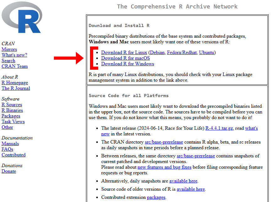
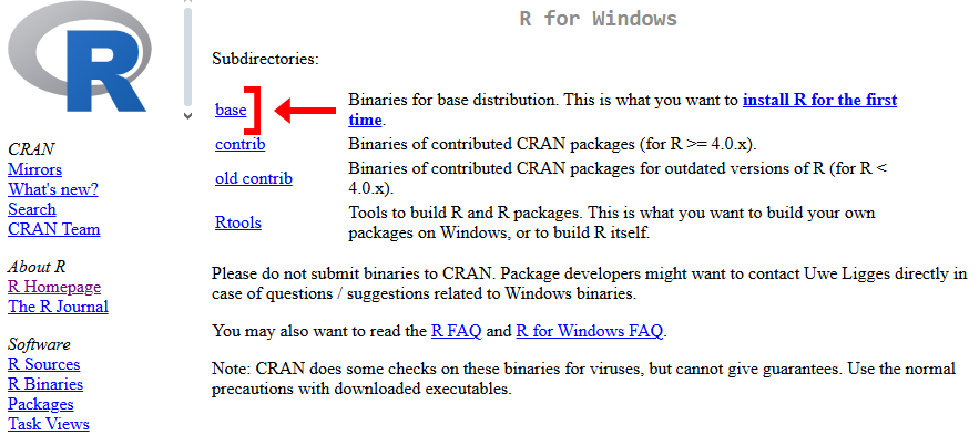
**First**, we need to install R. Click the button below and click "Download and Install R". Choose your OS. For Windows you need to download "**base**"; for MacOS and Linux you have to choose the version of your OS. Install.
[Download R](https://cran.rstudio.com){.btn .btn-primary .btn role="button" target="_blank" style="width:200px"}
Step one
For windows:
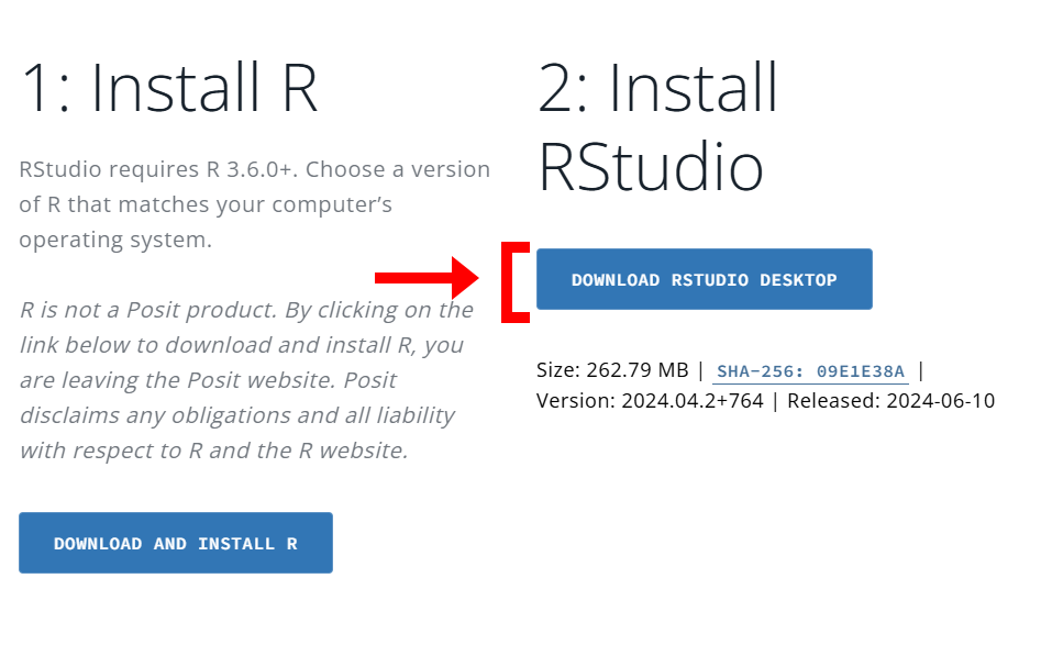
**Second**, we need to install RStudio. Click the button below and click "Download RStudio Desktop". You will be redirected to your version automatically. Install.
[Download RStudio](https://posit.co/download/rstudio-desktop/){.btn .btn-primary .btn role="button" target="_blank" style="width:200px"}
Step two