# Review of the previous week
::: callout-note
## Review
Load the `tidyverse` library and sipri dataset
```{r}
#| message: false
library(tidyverse)
sipri = read.csv("data/sipri.csv")
```
Using `GGally` library, visualize the relationship between `Import` and `Regime` variables
```{r}
```
Set up a linear model. Predict `Import` by `Regime`.
```{r}
```
What is the reference category in this case?
```{r}
```
Using `relevel()`, set the reference category to `Minimally Democratic`
```{r}
```
Set-up the model again, and plot the `ggpredict()`. Did anything change?
```{r}
```
Extract the model information using `tidy()` function from `broom` library.
```{r}
```
Visualize the effects plot. Is it different to the plot generated by `ggpredict()`?
```{r}
```
:::
# Review of the homework
- Although the DV in the problem set was binary, we asked to set up a linear model. We didn't discuss it, but it's called Linear Probability Model. Alternative is logistic regression, which we have not covered yet.
# Agenda
- Replicating a paper, applying tools we learned
# The paper
Today we are replicating George Ward's paper.[^1]
[^1]: The material for this lab is based on the University of Mannheim's Quantitative Methods class. The paper replicated is Ward, G., 2020. Happiness and voting: Evidence from four decades of elections in Europe. *American Journal of Political Science*, 64(3), pp.504-518.
Ward is interested in a quite straightforward question: Is subjective well-being a predictor of election results?, or more specifically: Do government parties get more votes when the electorate is happy? Ward uses observational data to find an answer to this question. He did both micro and macro level analyses. We will focus on the macro level analysis.
Part of his data comes from a great source -- [Eurobarometer](https://www.gesis.org/en/eurobarometer-data-service). Feel free to explore in your free time.
First, load the data.
```{r}
load("data/ward2020.Rdata")
head(dta)
```
The variables are the following:
- `country` = country
- `year` = election year
- `vote_share_cab` = % votes won by cabinet parties
- `satislfe_survey_mean` = Life Satisfaction, Country-Survey mean (1-4 scale)
Let's pause for a second, and think about the data structure.
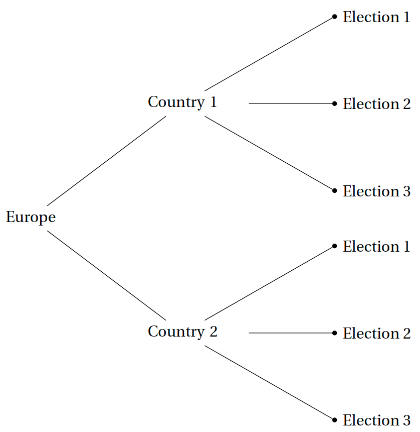
Say, you find a correlation between citizen’s happiness (`satislfe_survey_mean`) before an election and the electoral outcome (e.g. `vote_share_cab`). Would you consider this as strong evidence for the claim that happiness causes voters to vote for incumbent parties?
There may be ommitted confounding variables. Because the data structure is hierarchical, we can think of potential counfounders on the country level (variables that vary between countries but not constant over time, e.g., GDP per capita) and on the election level (variables that vary within countries, e.g. voter turnout).
Thus, we need to control for these confounding variables.
# Simple linear regression model
Our dependent variables is vote share of cabinet parties (`vote_share_cab`) and we are interested in the effect of happiness (`satislfe_survey_mean`).
```{r}
lm_pooling = lm(vote_share_cab ~ satislfe_survey_mean, data = dta)
```
Present the summary.
```{r}
```
The model can be written as follows:
$$
Y_{it} = \beta_0 + \beta_1X_{it} + u_{it}
$$
Subscripts:
- $i$ indicates countries.
- $t$ indicates time points, i.e. elections.
This approach is sometimes called **complete pooling**, because we throw all the data from all the countries and all the elections into one and the same pool. In other words: we ignore the data structure in the model specification.
Take a moment to plot the regression using `ggplot()`.
```{r}
#| eval: false
ggplot()
```
# Regression with fixed effects
There are different sorts of fixed effects, broadly speaking unit and time fixed effects. Let’s discuss it step-by-step.
## Unit fixed effects
First of all, the fixed effects should be of class `factor()`. Let's check it and correct if needed.
```{r}
class(dta$country)
dta$country = as.factor(dta$country)
```
Unit fixed effects regression models can be very useful to solve one of the problems we already identified: omitted confounders on some higher level unit of observation. This higher level unit, in our case, are countries. Thus, let's add **country fixed effects**. Notably, the variable `satislfe_survey_mean`.
```{r}
fe_model = lm(vote_share_cab ~ satislfe_survey_mean + country, data = dta)
summary(fe_model)
```
Let's visualize the model. Load the `ggeffects` library.
```{r}
library(ggeffects)
```
To simplify the perception, let's choose only the following countries: `AUT, DNK, IRL`. You can see the effect of adding the `country` variable quite vividly, right? Compare it to the previous graph.
```{r}
#| eval: false
ggpredict(..., terms = c("...", "... [AUT, DNK, IRL]")) %>%
plot()
```
Including country fixed effects has the following pros and cons:
- **Advantage**: Confounders that only vary between countries are of no more concern.
- **Disadvantage**: We lose all the higher level information. So if we were interested in why governing parties in country A seem to systematically receive more votes than governing parties in B, then we cannot answer them anymore as soon as we include country fixed effects. Why? Perfect colinearity between country fixed effects and time-invariant country characteristics (e.g, political system)
## Two way fixed effects
Now, let's add year fixed effects. Usually, when we have two fixed effects, we refer to it as **two way fixed effects**.
Again, the fixed effects should be of class `factor()`. Let's check it and correct if needed.
```{r}
class(dta$year)
dta$year = as.factor(dta$year)
```
Just as country fixed effects help us to account for all unobserved confounders that only vary across countries (but not within countries), time fixed effects help us to account for all unobserved confounders that only vary across time (but not within time, i.e. between countries at one point in time).
```{r}
twfe_model = lm(vote_share_cab ~ satislfe_survey_mean + year + country, data = dta)
summary(twfe_model)
```
Let's visualize to get the sense of what's going on. Check the following countries `AUT, DNK, IRL` in the following years `1987, 1992, 2011`. As it is a fixed effects model, we can interpret the same style as "holding everything else constant, on average one unit increase ...".
```{r}
ggpredict(twfe_model, terms = c("satislfe_survey_mean", "country [AUT, DNK, IRL]", "year [1987, 1992, 2011]")) %>%
plot()
```
Usually, we do not report estimates for the fixed effects. You would expect to see something like this:
```{r}
#| message: false
library(modelsummary)
modelsummary(list("Pooled Model" = lm_pooling,
"Fixed Effects Model" = fe_model,
"Two-Way Fixed Effects Model" = twfe_model),
coef_omit = "country|year",
stars = TRUE,
gof_omit = "AIC|BIC|Log.Lik.|F|RMSE",
add_rows = data.frame(term = "Fixed effects",
pooled = "N",
fixed = "Y",
twfe = "Y"))
```
## Including control variables
By including country and year fixed effects, we made sure that our effect estimate is not biased due to unobserved confounders that are time-invariant on the country level in a given year. However, we still need to think about potential **time-variant** confounders we need to control for. Take a moment to think this through.
Here, we are back in the familiar game: we must think about potential covariates, try to get the data and include them in our model. Ward includes a series of control variables:
- `parties_ingov` = Number of parties in government
- `seatshare_cabinet` = % seats held by governing coalition
- `cab_ideol_sd` = Gov Ideologial Disparity (Standard deviation of government party positions on left-right scale)
- `ENEP_tmin1` = Party Fractionalisation - Last Election (Gallagher Fractionalization Index)
Let us set up the model.
```{r}
twfe_controls_model = lm(vote_share_cab ~ satislfe_survey_mean + year + country + parties_ingov + seatshare_cabinet + cab_ideol_sd + ENEP_tmin1, data = dta)
```
By now, the summary below is unreadable.
```{r}
#| eval: false
summary(twfe_controls_model)
```
Let's play around the `modelsummary()` to include the most important information.
```{r}
modelsummary(twfe_controls_model,
coef_omit = "country|year",
stars = TRUE,
output = "markdown")
```
However, often authors present only the main explanatory variable. You should mention your controls, but you don't have to report it directly (usually, in this case the extended table goes to appendix). Let's present all of the models. And customize the display. This is what you can see in Table 1(column 1) of the article with one difference. The author standardized numeric variables. Why would you standardize the variable in this case?
```{r}
modelsummary(list("Pooled Model" = lm_pooling,
"Fixed Effects Model" = fe_model,
"Two-Way Fixed Effects Model" = twfe_model,
"Two-Way Fixed Effects Model w Controls" = twfe_controls_model),
coef_rename = c("(Intercept)", "Well-Being"),
coef_omit = "country|year|parties_ingov|seatshare_cabinet|cab_ideol_sd|ENEP_tmin1",
stars = TRUE,
gof_omit = "AIC|BIC|Log.Lik.|F|RMSE",
add_rows = data.frame(term = c("Fixed effects", "Conrols"),
pooled = c("N", "N"),
fixed = c("Y", "N"),
twfe = c("Y", "N"),
twfe_c = c("Y", "Y")))
```
# Exercises
Let's explore Comparative Political Dataset. Take a look on their [codebook](https://cpds-data.org/wp-content/uploads/2024/11/codebook_cpds.pdf).
Load the data from the Canvas, or by clicking this button:
Using the `readxl` library, load the dataset.
::: {.callout-tip icon="false"}
## Solution
```{r}
#| eval: false
library(...)
cpds = read_excel("data/cpds.xlsx")
```
:::
The dataset contains the information on political systems of different countries in different years. Let's explore the following variables:
- `country` name
- `year` of the observation
- `gov_right1` - cabinet posts of right-wing parties in percentage of total cabinet posts
- `outlays` - total outlays (disbursements) of general government as a percentage of GDP
Subset these variables from the dataset.
::: {.callout-tip icon="false"}
## Solution
```{r}
#| eval: false
cpds_sub = ...
```
:::
Visualize the distribution of the `gov_right1` variable.
::: {.callout-tip icon="false"}
## Solution
YOUR SOLUTION HERE
:::
Check the class of `outlays` variable. Using the `head()` function, explore the first 6 rows of the `cpds_sub` dataframe. Does the class seem right? If not, correct.
::: {.callout-tip icon="false"}
## Solution
YOUR SOLUTION HERE
:::
Using `ggpairs()` from `GGally` library, explore the distribution of `gov_right1` and `outlays` variables, and their relationship. What do you notice?
::: {.callout-tip icon="false"}
## Solution
YOUR SOLUTION HERE
:::
Set up a linear model. Predict `gov_right1` by `outlays`. Interpret the results.
::: {.callout-tip icon="false"}
## Solution
YOUR SOLUTION HERE
:::
Using $\LaTeX$ write out the formula of the regression. Don't forget about the subscripts.
::: {.callout-tip icon="false"}
## Solution
YOUR SOLUTION HERE
:::
Include the `year` fixed effects. Make sure it is of right class. Does the result hold? Interpret the coefficient for `outlays`.
::: {.callout-tip icon="false"}
## Solution
YOUR SOLUTION HERE
:::
Now, let's set up a two-way fixed effect. Introduce the `country` fixed effects. Make sure it is of right class. Did the result change? Interpret the results for `outlays`.
::: {.callout-tip icon="false"}
## Solution
YOUR SOLUTION HERE
:::
Let's explore this model. Using `ggpredict()` plot the terms in the following order: `outlays`, `country`, `year`. Choose the following countries: `Austria, Canada, Sweden`, and the following years: `1961, 1996, 2016`. Do the slopes and confidence intervals explain the significance of the `outlays` variable?
::: {.callout-tip icon="false"}
## Solution
YOUR SOLUTION HERE
:::
Using `modelsummary()`, present the results for all the models. Don't forget to customize the output.
::: {.callout-tip icon="false"}
## Solution
YOUR SOLUTION HERE
:::
# Check List
I understand that the structure of the data can be different
I know what pooled regressions means
I know what the fixed effects types are
I am not scared of such terms as two way fixed effect (TWFE)
I know how to present only selected cases using `ggpredict()`
I know how to customize `modelsummary()`